New Definition of Probability
January 11, 2021 by Asad Zaman
{bit.ly/rsia08a} Lecture 8A of Real Statistics: An Islamic Approach, provides answers to the question of “What is Probability?”. An article by Alan Hajek in Stanford Encyclopedia of Philosophy lists six major categories of definitions. Many more are possible if causality is also taken into account. These definitions conflict with each other, and face serious problems as interpretations of real-world probabilities. The basic definition of probability we will offer in this lecture falls outside all of these listed categories. Before going on to present it, we briefly explain why the currently dominant definition, based on limiting frequency, does not make sense
1 Emergence of Probability in Europe
According to Ian Hacking’s account in the Emergence of Probability, modern concepts of probability emerge in the middle of the 17th Century Europe, and have not evolved substantially since then. He explains that these formulations were shaped by (now forgotten) historical contexts which constrained the space of possible theories. This explains why satisfactory definitions of probability are not available even in the beginning of the 21st Century. To vastly oversimplify, we provide TWO major reasons why attempts to define probability went astray.
ONE: Colin Turbayne, in his superb but neglected book “Myth of Metaphor”, has documented how Newtonian metaphor of the world as a machine, governed by deterministic laws, replaced an earlier metaphor of the world as an organism. In a deterministic world, there are no chance events. This constrains probability to be an aspect of our ignorance regarding the laws governing the universe. This precludes the existence of probabilities in external reality.
TWO: Empiricist philosophies originating with Hume and culminating in Logical Positivism deny the relevance of unobservables to science. Probability is intrinsically concerned with what might have happened, and hence not definable in terms of what did happen
2 A New Concept of Probability:
We will now define probability via a new framework, for use in this course. Consider a random event such as a coin flip. Our definition is Chronological – it takes into account a central feature of probability not available in the major definitions. Probability exists and is well-defined BEFORE the coin is flipped.
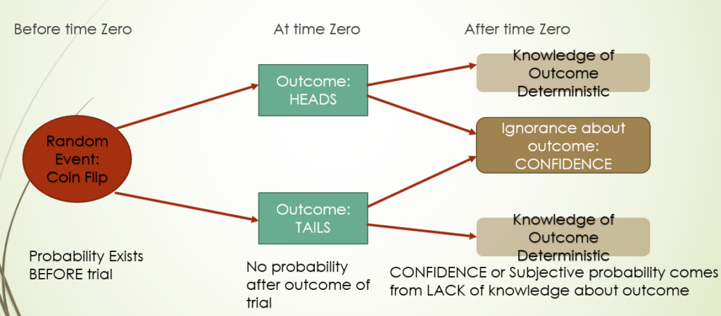
We understand this probability as a “propensity”, a feature of external reality having to do with the coin and how it is flipped. After the flip, an outcome occurs – normally either Heads or Tails. When the outcome occurs, the probability is EXTINGUISHED. We are now in one of two possible mutually incompatible worlds, as depicted in the diagram above. In either of the two worlds, we cannot talk about the Probability of Heads or Tails, because the uncertainty has been resolved, and a definite outcome has occurred. However, suppose that I do not know which of the two outcomes occurred. In this case, my knowledge of the pre-event probability gives me information, which can be formalized using the term “CONFIDENCE”. We can say that I have confidence level of 50% that Heads occurred, and similarly for Tails. This confidence is subjective – personal to me – because of my ignorance about what happened. Someone who knows what happened would not share my personal assessment at all. Confidence comes into being after probabilities are extinguished, and does not exist prior to the occurrence of the random event.
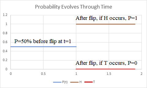
To express this formally, use X to denote a random variable, representing a coin flip. Traditional notation writes P(X=Heads)=P(X=Tails)=1/2 for fair coin. However, this ignores the temporal nature of probability. For each random variable, there is a time of OCCURRENCE, a time at which the random variable takes a particular outcome and uncertainty is resolved. This must be an essential part of the description of the random variable. Let us write X[s] for a random variable which is uncertain upto time s. Then the coin flip occurs at time s and results in a specific outcome: Heads or Tails. In talking about Probability, we must also mention the time at which probability is being evaluated, since this probability changes with time. Let use P(t) to denote probability at time t. Then the simplest picture of the probability of a coin flip is depicted in the following function: P(t){X[s]=Heads}:
Here, the coin is flipped at time s=1. Prior to t=1, probability of Heads is 0.5. After t=1, this probability is either 100% when Heads occurs as an outcome of the coin flip, or 0%, when Tails occurs.
This definition incorporates several features not available in any of the current major definitions of probability. As explained by Hacking, conceptions of probability were constrained by historical context, and have not succeeded in liberating themselves from these original constraints. In particular, understanding of causality is closely connected with the ability to create imaginary worlds, which are different from, and yet similar to, our experienced reality. In this conception of probability, the coin flip creates two possible worlds, which differ from each other only is this single respect – in one world, the coin came out heads, while in the other it came out tails. As time progresses, differences created by this branch may be extinguished, or may be amplified. For example, if an important decision (like choosing strategies or teams) is linked to the coin flip then difference in outcomes could lead to further differences. But all these topics, and connections to counterfactuals and causality, are not relevant to the present lecture. Here we aim to provide an elementary introduction to probability for beginning students.
3 Conjectural Probability
In the picture of probability above, a crucial element is missing. How do we assign probabilities to the two branches? How do we know that Head and Tails are equally likely and have 50% probability? If the event is Rainfall or Clear Weather tomorrow, what are the probabilities to be assigned to the two branches?
As per critical realist philosophy, scientific theories are conjectures about the hidden structures of reality. These can never be verified directly, because these structures remain unobservable. But sufficiently good matches between predictions of these theories and observed outcomes give us indirect confirmation, and a reason to trust these theories. Along these lines, the probabilities ascribed to the branches represent a conjecture about reality, which can never be verified to be true.
According to positivist dogma, a sentence with unverifiable truth value is meaningless. The grip of binary logic has made this way of understanding probability inaccessible within European intellectual traditions which gave birth to the modern concepts of probability. We now illustrate conjectural probability with examples.
3.1 “Fair” Coin
A Coin Toss if often used for choosing at random among two options. The hypothesis of “fairness” is a conjecture that the two possible outcomes are equally likely. The physical symmetric structure of the coin, the circumstances of tossing, and historical experience, all provide evidence for the conjecture that P(Heads)=P(Tails)=50%, prior to the toss. After the toss on of the two outcomes occurs, and probability is extinguished. If a person is IGNORANT of outcome, he can have SUBJECTIVE probability. He can have CONFIDENCE 50% that Heads occurred, and similarly CONFIDENCE 50% that Tails occurred.
3.2 Equal Skill in a Game
Suppose we CONJECTURE that two players A & B have EQUAL skill. One meaning of “equal skill” is that both have equal chances of winning a particular game. Thus the conjecture of equal skill leads us to assign probabilities: P(A wins)=P(B wins)=50% if DRAW is not a possible outcome. if DRAW is possible, then P(A wins)=P(B wins)= 50% of (1-P(DRAW)). Conjectural Probability created by adding a THEORY about real world and attempting to see if it matches the observations. Note that we may believe the theory to be obviously false. The point of putting down the theory is to reject it by using data, providing an empirical proof that one of the two players is more skillful.
3.3 Drug Versus Placebo
Take two groups of patients – Treatment & Control Group. Match the patients in pairs, assigning one control to one treatment: T1 to C1, T2 to C2, … . Attempt to match the pairs on all relevant factors. Give Drug to treatment group and Placebo to control group. We CONJECTURE that the Drug has no effect (Drug equivalent to Placebo). As a consequence, difference in Outcomes is purely random – that is, the two outcomes (T1 cured, C1 not) and (T1 not, C1 cured) are equally likely. We can use predictions of this conjectured probability to assess whether or not the conjecture is in conformity with empirical evidence. Again, we will normally be interesting in a statistical REJECTION of this conjecture. That would give us empirical evidence for the efficacy of the drug.
3.4 Drawing Straws:
There are twelve people on a boat which gets caught in a storm. They believe that the storm has been sent to punish a guilty person who is fleeing the scene using the boat. They decide to draw straws to determine who is guilty. Twelve straws of equal length are taken, and one of them is broken off at one end. The break is concealed, and the bundle held out to all parties sequentially. The one who ends up drawing the short straw is deemed to be guilty and thrown off the boat. The probability conjecture is that all straws have equal probability of being drawn. Under this hypothesis, it can be shown that all parties have equal chances 1/12 of being found guilty.
3.5 Independence and ESP
Two people are given a deck of cards. One of them is asked to choose one of them at random, put it aside, and pick a second one, and continue through the deck in this way until the end. The second person is asked to guess the color of the card and record his guess (Red or Black). At the end of the experiment, we will have 52 pairs of the type (R,R) (R,B) (B,R) and (B,B). The conjecture that the guess and the draw are independent leads to equal probability for all 4 pairs. In contrast, if the second party has ESP, then (R,R) and (B,B) will occur more often than they should under independence. We can check the data to see if it is in strong conflict with the conjecture of independence, as evidence for ESP.
3.6 The Vietnam Draft Lottery
The Vietnam Draft Lottery was instituted to create a fair way to choose how to send young men to kill Vietnamese, and possibly die in the process. This was done by randomly choosing from among the 366 days of the year, and also randomly choosing between the letters of the alphabet A,B,…,Z, to decide on ranking of young men, according to birthdate and initial letters of the names. Under the conjecture that all dates and names had equal probability, all of the young men in the target age range would have equal chances of being picked. There was substantial controversy regarding this, and ultimately it was concluded that the process by which the dates had been picked did not give equal chances to all days of the year.
4 Confusion about the Bayes Rule
Our conception of probability and confidence allows us to resolve a dilemma which has been a source of controversy for centuries. Consider an urn containing three balls, two of which are White while one is Black. At time s=1, we make the first random draw D1 from the box. Thus P(D1=W)=2/3 and P(D1=B)=1/3. Here we adopt the simplifying convention that when time is not mentioned for probability or for the random variables then both times are assumed to be PRIOR to the occurrence time.
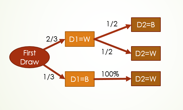
At time s=2, we make the second random draw. The probabilities for this draw are as shown in the diagram. If D1=W then remaining balls are WB and both have equal chances of being drawn. If D1=B than both remaining balls are white, so the only possibility is D2=W.
The branches on the diagram leading to outcomes of the second draw D2 have conditional probabilities. These are probabilities based on OUTCOMES of D1. The uncertainty associated with the first draw has been extinguished, and a particular fixed outcome – D1=W or D1=B – has occurred. Suppose we want to compute the probability of a sequence of draws, such as D1=W and D2=W. This probability changes with time. At t=2, all probabilities are extinguished: P(2){D1=W & D2=W} = 100% or 0%, depending on the outcomes of the two draws. At t=1, uncertainty only attaches to the second draw. The outcome of D1 has already occurred. There are two possibilities – either P(1){D2=W}=50%, when D1=W occurred, OR P(1)(D2=W)=100% when D1=B occurred.
To understand the Bayes controversy consider calculating the probability at time t=0 of a sequence of draws such as D1=W and D2=W. It is easily seen that
P(0){D1=W & D2=W} = P(0){D1=W} x P(1){D2=W|D1=W} = 2/3 x 1/2 = 1/3
Here the conditional probability written as P(1){D2=W|D1=W} has a natural interpretation. At time t=1, the first draw has OCCURRED, and an outcome has been observed. All probabilities going forward depend on which outcome occurred, and so this must be specified as the condition, to allow computation of the probability.
The Bayes formula arises when we fail to keep track of time while evaluating probabilities. The formula above is written in traditional notation as P(A & B) = P(A) x P(B|A), and this is taken to be a universal law of probability. When B follows A in time, this makes sense, and corresponds to our formula. However, now consider reversing the roles of A and B. This gives P(A & B) = P(B) x P(A|B). If A and B are contemporaneous events, this would work fine. But in the present case the second formula can be written as follows, without indicating time:
P(D1=W & D2=W) = P(D2=W) x P(D1=W|D2=W)
This has the un-natural conditional probability which asks about the probability that D1=W given that D2=W. At what time is this probability being evaluated? The natural time is t=2, when the outcome of the second draw has occurred and is W. But then D1 has also occurred and has a known outcome. Probabilities associated with D1 have been extinguished. So, standing at time t=2, we cannot ask about probabilities of events which took place at an earlier time t=1. The chronologically sequenced events are no longer symmetric, and the conditional probability which makes perfect sense in the natural direction of time flow makes no sense when we reverse the direction of time.
2 ONCLUDING REMARKS
Ian Hacking in “The Emergence of Probability” writes that:
The preconditions for the emergence of probability determined the space of possible theories about probability. That means that they determined, in part, the space of possible interpretations of quantum mechanics, of statistical inference, and of inductive logic.
That is, historical circumstances in Europe determined the ways of thinking about probability which emerged – and EXCLUDED many other possible ways of framing thought about probability. Other histories could lead to other concepts of probability, and Hacking mentions tantalizing alternatives from Indian history. In this lecture, we have provided an alternative framework to conceptualize probability, and to resolve the vexing conflict between subjective and objective probability.