This is the second in a sequence of lectures about regression models and methodology. These regression models are central in econometrics. Current methodology underlying these models makes them completely useless for learning about the real world. To learn how and why, we first discuss the differences between nominalist and realist methodology for science.
Underlying Philosophy of Science
Many important structures of the real world are hidden from view. However, as briefly sketched in previous lecture on Ibnul Haytham: First Scientist, current views say that science is only based on observables. Causation is central to statistics and econometrics, but it is not observable. As a result, there is no notation available to describe the relationship of causation between two variables. We will use X => Y as a notation for X causes Y. Roughly speaking, this means that if values of X were to change, then Y would have a tendency to change as a result.
This is not observable for two separate reasons. ONE because it is based on a counterfactual. In another world, where the value of X was different from what was actually observed in our current world, this change would exert pressure on Y to change. TWO X exerts an influence on Y, but there are other causal factors which are also involved. Thus Y might not actually change in the expected direction because the effect of X might be offset by other causal factors which we have not accounted for. For both of these reasons, causality is not directly observable.
Achieving Conceptual Clarity
The standard approach to statistics and econometrics is based on a huge number of confusions. The same word is used for many different concepts. To clear up these confusions, we need to develop new language and notations. We start by distinguishing between three different types of ideas:
- O-concepts refer to the Observables.
- M-concepts refer to a model for the data
- R-concepts refer to the Real World
R-concepts refer to factors in the real world, and causal effects which link them. For example, Household income could be one of the factors which causally influences consumption decisions. Let us use HI* and HC* to denote real world household income and consumption for some particular household. We will use => to denote causation: HI* => HC*. A household income-expenditure survey obtains measures HI and HC of HI* and HC*.
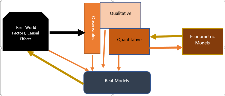
We will use this notational convention to distinguish between real world concepts and their observable counterparts. An econometric model attempts to find a model which fits data on HI and HC. A real model uses the data on HI and HC as clues to tease out causal relationships within real world variables HI* and HC*.
To illustrate how real-world models are constructed, we go through a hypothetical example close to reality. We start with a hypothesis about a real world causal relationship; for example, HI* => HC*. Causal relationships are unobservable, so no direct confirmation is possible. However, examination of data on HI and HC can provide indirect evidence confirming or disconfirming the hypothesis. There are three main possibilities: HI* => HC*, HC* => HI*, and HC* ^ HI*. The last is the standard symbol for independence, but since this is not generally available, we will also use || double vertical bars as a replacement notation: HC* || HI* means that the two variables are independent – neither causes the other. Note that there would be many other possibilities, such as bidirectional causality, or causal effects mediated through intervening variables, but we are considering the simplest possible cases, to start with.
The data can provide us with evidence regarding these causal relationships. If we see large variations in HI* and very little in HC*, we would be tempted to reject the causal hypothesis that HI* => HC*. This might be the case in an ideal Islamic society, where everyone follows simple lifestyles, regardless of income levels. If, on the other hand, we see that consumption levels increase with income, this would suggest that our hypothesis may be true. But, we always need to check for reverse causation. Suppose for example that people are accustomed to different lifestyles, and they earn to support their lifestyle. Those who desire higher consumption levels will be driven to earn higher incomes. In this case the causal direction will be the reverse: HC* => HI*. There are many different ways that we can judge the direction of causation, according to availability of data, or using experiments which vary income.
Regression: Most widely used model
Fisher introduced the idea of making an assumption that data is a random sample from a hypothetical imaginary distribution, in order to simplify data analysis. Regression extends this idea to two or more variables. It is based on LARGE number of FALSE assumptions. As we have seen, a nominalist methodology has no difficulties with false assumptions. It does not matter if Model doesn’t correspond to Reality. We only check FIT between model & data. In contrast to this, REALISM says that False assumptions lead to false results; that is our premise in this course on Real Statistics.
A Standard Course Introduces Assumptions of the regression model with minimal explanation. The goal is never to analyze or understand these assumptions, or to assess if they are true. The assumptions just provide us with the mathematical tools required to do data analysis. The standard course USES the assumptions to do complex mathematics required to setup and estimate regression models. A whole SEMESTER of work is involved in learning the MECHANICS of regression. Since nearly all regression models are false, all of this is useless. In this course, we will study Regression Models from OUTSIDE. That is, we will discuss how regression models are setup and estimated, without discussing the mechanical and mathematical details.
Causality:
As discussed earlier, causality is not observable. We can see that Y happens after X, and but not that Y happens because of X. Because of this, the positivist methodology of econometrics makes no mention of causality. Yet, causality is central to understanding regression models, and also, why they fail. We have already introduced the notation that “X => Y” reads “X causes Y”. What does this mean? Changes in X lead to changes in Y. The relationship is DIRECT. If we have X => W => Y this is NOT equivalent. In this situation, W is a MEDIATOR – it mediates the relation between X and Y. Other causal factors may be present. X => Y and Z => Y is possible and often the case. Other chains of causation may be present. X => Y and ALSO X => W => Y can BOTH hold. However, we will assume that there is no circular causation. We cannot have X => Y and Y => W => X. Although such situations may be possible, we ignore them for simplicity in our initial approach to causality. With this notation in place, we can now discuss the assumptions of the regression model.
Assumptions of the Regression Model
Regression starts by identifying a dependent variable Y, which we wish to “explain”. The regressors are a set of variables X1, …, Xk to be used in explaining Y. Since the notion of “explain” is never explained, the meaning of these fundamental assumptions never emerges clearly. In this lecture, we will only consider the case of a single regressor X. The key assumption is one of a causal relationship between X and Y: X => Y. This is referred to as the Exogeneity of X, but there is no real understanding of what this means. Next we assume a LINEAR relation between Y and X, and some other factors which are not known:
Y= bX + F1 + F2 + F3 + … + Fn
If we aggregate the unknown factors into an error term, we get the regression model: Y = bX + ErrY. An important assumption is that ErrY is INDEPENDENT of X. We will use =/> to mean “does not cause”. Then the independence assumption X || Fi means X =/> Fi and also Fi =/> X, where Fi are the unknown factors which go into the error term. To run a regression, we will need multiple data points. Then, an additional assumption is that ErrY is independent across time or sector. We also have the standard Fisherian assumption: ErrY is random sample from common distribution. If we let M be the common mean of this unknown distribution, we can write the regression equation as Y = M + bX + (ErrY-M). In this equation we have a constant term, and the new error term is ErrY’ = ErrY-M. This error term has mean 0.
- What is the BASIS for these assumptions? NONE.
- Can we expect them to be roughly valid? NO!
These are all INCREDIBLE & BIZARRE assumptions – it is almost impossible to think of situations where they would hold. Edward Leamer analyzed the regression model and stated The Axiom of Correct Specification: Regressions produce good results ONLY IF ALL ASSUMPTIONS HOLD. Failure of any one of the assumptions can lead to dramatically wrong conclusions. Many examples of such failure can be demonstrated in highly regarded papers published in top journals. The biggest problem is that regressiom models create confusion about causal effects in minds of students. This makes it impossible for them to use data to arrive at sensible conclusions about reality.
Yule fitted the first regression model to data in 1896, and failed to reach any conclusions regarding the problem he attempted. Hundred years later, in a centenary article, Freedman (1996) wrote that we have tried this methodology for a century, and it has failed to produce good results. The time has come to abandon it. This is precisely our point of view. Regression models have failed, and should be abandoned. In this chapter, we will describe the methodology and its failures. Later we will develop alternative, superior methodologies, based on a REALIST approach, which does not allow to make false assumptions freely, to fit the data. With this as background, we now turn to regression models.
Regression: Fitting lines to data
- Why are we fitting a line to the data?
- What does the fitted line MEAN?
- How do we calculate which line fits best?
- What will be done with the regression analysis?
In real world situations, there are a number of possible DIFFERENT uses for fitting lines. The interpretation of the LINE depends greatly on real world context which generates the numbers, and the PURPOSE for which this analysis is being done.
Measuring Serum K levels in Blood:
The data we analyze is two ways of measuring Serum kanamycin levels in blood. Samples were drawn simultaneously from an umbilical catheter and a heel venipuncture in 20 babies – this is a real data set taken from Kaggle. The data set and a graph of the data are given below:
| Baby | Heelstick | Catheter |
| 1 | 23 | 25.2 |
| 2 | 33.2 | 26 |
| 3 | 16.6 | 16.3 |
| 4 | 26.3 | 27.2 |
| 5 | 20 | 23.2 |
| 6 | 20 | 18.1 |
| 7 | 20.6 | 22.2 |
| 8 | 18.9 | 17.2 |
| 9 | 17.8 | 18.8 |
| 10 | 20 | 16.4 |
| 11 | 26.4 | 24.8 |
| 12 | 21.8 | 26.8 |
| 13 | 14.9 | 15.4 |
| 14 | 17.4 | 14.9 |
| 15 | 20 | 18.1 |
| 16 | 13.2 | 16.3 |
| 17 | 28.4 | 31.3 |
| 18 | 25.9 | 31.2 |
| 19 | 18.9 | 18 |
| 20 | 13.8 | 15.6 |
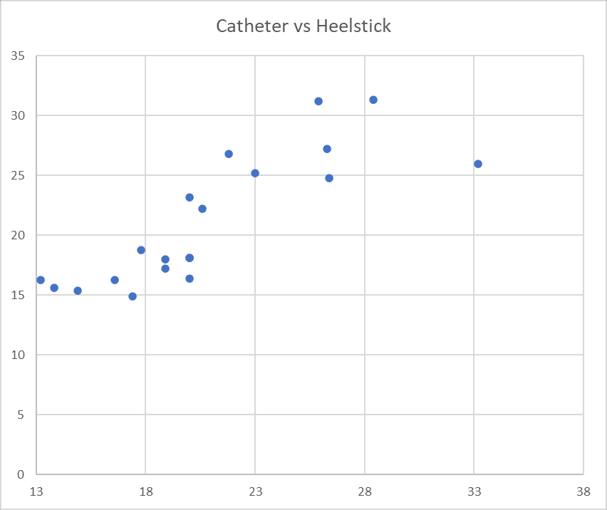
The data and the graph show a rough correspondence between the two measures, which is what we expect to see. Both Cath and Heel are measures of the same unknown quantity K, the serum K levels in the blood of the baby.
The data is relevant to the analysis of a meaningful question. Are the two measures equivalent? Do they provide us with an accurate measure of the true Serum Kanamycin levels (K) in the baby’s blook? The unobserved real variable K generates the two measures C and H: K => C and K => H. Because both are caused by K, we expect to see high correlation between the two. BUT there is no causal relationship: C =/> H and also H =/> C. Neither measurement causes the other. A reasonable representation of the underlying structure is: C = K + ErrC and H = K + ErrH. This is A GOOD model because it matches underlying unobserved reality. The errors are meaningful – they represent the errors created by assuming that the sample is representative of baby’s blood. As we will soon see, regression analysis cannot use either of these correct structural models because the involve the unknown and unobserved K.
Before turning to a regression, we do a little common-sense analysis of the data. It is well known that given two erratic but independent measurements, an average of the two will give us a more stable and accurate measure. While K cannot be measured, if we define K* as the average of the two measures we have – K* = (C+H)/2 – then K* will provide a better approximation to the underlying true K than either of the two measures C and H. Using this idea as the basis, we construct a table of values for K* and also plot the errors – the deviations from K* – of the two measures below.
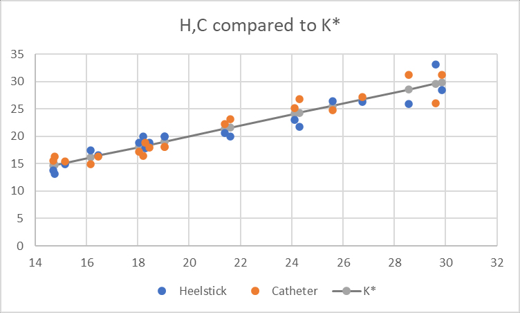
The X-axis is our estimated value K* of K. On the Y axis we plot K* and compare it with the two measures H and C. As we can see, both measures are closely matched to K*, so the data conforms to our intuitions regarding the two measures H and C, and the underlying unobserved K. There are few things we can learn from this data analysis. First we present the “errors” in the measures C and Y and measures of K*. Note that these are NOT the TRUE errors, because the true value of K is unknown. Instead, we analyse ErrC* = C-K* and ErrH* = H=K*
| K* | ErrH | ErrC |
| 14.7 | 0.9 | -0.9 |
| 14.75 | 1.55 | -1.55 |
| 15.15 | 0.25 | -0.25 |
| 16.15 | -1.25 | 1.25 |
| 16.45 | -0.15 | 0.15 |
| 18.05 | -0.85 | 0.85 |
| 18.2 | -1.8 | 1.8 |
| 18.3 | 0.5 | -0.5 |
| 18.45 | -0.45 | 0.45 |
| 19.05 | -0.95 | 0.95 |
| 19.05 | -0.95 | 0.95 |
| 21.4 | 0.8 | -0.8 |
| 21.6 | 1.6 | -1.6 |
| 24.1 | 1.1 | -1.1 |
| 24.3 | 2.5 | -2.5 |
| 25.6 | -0.8 | 0.8 |
| 26.75 | 0.45 | -0.45 |
| 28.55 | 2.65 | -2.65 |
| 29.6 | -3.6 | 3.6 |
| 29.85 | 1.45 | -1.45 |
The three errors highlighted in red are the largest errors. All other errors are within 2 units of K*. From this analysis, we could conclude that the two measures are aligned, and both come within 2 units of the true K about 85% of the time. Occasionally, larger errors like 2.5 or even 4 can occur. One could go further by examining the particular cases of large errors to try to identify the source of the error. A real analysis always goes beyond the data, to try to understand the real world factors which generate the observations. Next, we turn to a regression analysis of this data set.
External Regression Analysis
A conventional course in regression analysis does the following:
- Learn assumptions of regression
- Use to create mathematical & statistical analysis
- Learn how to estimate regression models, & properties of estimators & test statistics
- Use this theory to interpret results of regression
Our point of view here is that the assumptions are nearly always false. As a result, the results are nearly always useless. So there is no point in learning all of this machinery, which take a lot of time and effort. Instead, we will teach regression from an external perspective. Running a regression involves doing the following tasks:
- Choose Dependent Variable Y
- Explanatory variables X
- Goal explain Y using X.
- Feed data to computer – we don’t investigate what happens inside the computer.
- Get regression output
- LEARN how to INTERPRET output.
A huge amount of time can be saved by learning how to drive the car, without learning the details of how the engine works. Accordingly, we proceed by running a regression analysis of the data on C and H.
We immediately run into a problem. Which of the two should be a dependent variable, and which should be the explanatory variable? Actually, the causal structure shows that both are dependent, while the independent variable is K. However, regression analysis does not allow the use of unobservables – we have no data on K. The nominalist philosophy says that we should ONLY use variables which are observable. Accordingly, there are only two possibilities, we can run a regression of H on C or of C on H. Both are wrong because both embody the wrong causal hypotheses, and end up giving us wrong and misleading results. We will examine the regression of H on C in greater detail. There are vast numbers of programs which we can use to run regressions; they all give similar results. Below, I present the results obtained from EXCEL:
B on C Heelstick on Catheter
Regression Statistics
Multiple R 0.832453
R Square 0.692978
Adjusted R Square 0.675921
Standard Error 2.904264
Observations 20
ANOVA
Df SS MS F Significance F
Regression 1 342.684 342.684 40.62765 5.29E-06
Residual 18 151.8255 8.434749
Total 19 494.5095
Coefficients Standard Error t Stat P-value Lower 95% Upper 95%
Intercept 4.210112 2.690918 1.564563 0.135096 -1.4433 9.863522
Catheter 0.786992 0.123469 6.373982 5.29E-06 0.527593 1.046392
This output is interpreted as follows.
Correlation & R-squared: Multiple R = 0.832453 ,R Square = 0.692978
In the nominalist theory, the most important aspect of regression is how well the model fits the data (not how well the model approximates truth). For this purpose, the correlation and its square are the most important measures in use. These measures the association between the dependent variable Y and the regressors, under stringent assumptions about the data.
This measure can give HIGHLY misleading results if assumptions are violated. Two variables which have no relation to each can have very high correlation. Also, two variables which are strongly related can have zero correlation. In this particular case, the two measures H and C are linearly related, so the correlation is a suitable measure of their association. The 83% correlation is high, and shows a fairly strong relationship between H and C. The R-square is SQUARE of correlation: 69.2% = 83.2% x 83.2%. This has the following standard Interpretation: 69.2% of the VARIATION in H variable can be explained by the C variable. This concept is meaningful ONLY under very strong assumptions rarely satisfied in real world applications. This comes from ANOVA analysis due to Fisher pursuing racist goals. Fisher wanted to explain variations in children use parents genes as causal factors, and to separate the contribution of genetics from the environment. However, this methodology does not actually succeed in achieving this goal.
Central Object of Regression is to FIT A LINE:
The most important goal of regression is to approximate the dependent variable as a linear function of the independent variables. The regression output estimates that H is a linear function of the C:
H = 4.21 + 0.79 C + err
A graph of this relationship is given below. The orange is the regression line, while the blue is the actual data.
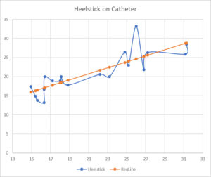
Visually, we can see that the data fits reasonably well to the line. This reflects the high correlation of 83%. However, this apparent linear pattern in data is not a good reflection of the TRUE relationship between these two variables H and C. The regression estimates don’t make sense. They have been derived under assumption that C is fixed, and H is caused by C. But this is not true.
A standard interpretation of this regression relationship would be that if we change C by one unit, then H would change by 0.79 units. This is NOT valid, because C is dependent on K and an Error ErrC. If we change ErrC – that is, the error of measurement – this will cause a change in C but not in K. Since K is the cause of H, changes in the error of measurement of C will not affect H. So the interpretation of 0.79 as the effect of changes of C on H is not correct. Similarly, none of the other statistics generated by regression make any sense, because the assumptions of the regression model are not satisfied.
The F-statistic for the Regression:
F 40.62765 Significance F 5.29E-06
We will end this lesson with an interpretation of the overall F-statistic for the regression as a whole. This is similar to the R-squared in being a measure of the overall goodness of fit between the data and the regression line. First we recall the meaning of the p-value, which is also called the significance level.
Significance Level: Suppose our null hypothesis is that a coin is fair. We flip it 100 times and observe 70 heads. The p-value measures how much this observation is in conformity with the null hypothesis. The p-value is defined to the probability of the observed event, together with ALL equal or more extreme events. Here more extreme means having lower probability. If X is the number of heads in 100 with 50% success probability on each trial, then the p-value of the observation 70 is P(X>=70)+P(X<=30) which is 2*3.92507E-05, an extremely low probability. This means that the event is highly unlikely under the null hypothesis. Because there is a high degree of conflict between the observed event and the null hypothesis that the coin is fair. So, we can reject the null hypothesis.
Now, we go back to the interpretation of the F-statistic. This is a test for the null hypothesis that all coefficients in the regression are 0. That is a=0 and b=0, so that there is no connection between the two measures H and C. The statistic of 40 with significance of 5.3E-06 means that this is highly unlikely. So, we can reject the null hypothesis of no connection between H and C. While the inference is correct (that is, there is a strong relationship between H an C), the reasoning which leads to this conclusion is wrong. Also, the p-value is meaningless, since the assumptions on which it is based are not valid.